Automatic Music Generation

Overview

Learn how to develop an end-to-end model for Automatic Music Generation Understand the WaveNet architecture and implement it from scratch using Keras Compare the performance of WaveNet versus Long Short Term Memory for building an Automatic Music Generation model

Table of Contents What is Automatic Music Generation? What are the Constituent Elements of Music? Different Approaches to Music Generation Using WaveNet Architecture Using Long Short Term Memory (LSTM) Implementation – Automatic Music Composition using Python

What is Automatic Music Generation?

Music is an Art and a Universal language.

I define music as a collection of tones of different frequencies. So, the Automatic Music Generation is a process of composing a short piece of music with minimum human intervention.

automatic music generation

What could be the simplest form of generating music?

It all started by randomly selecting sounds and combining them to form a piece of music. In 1787, Mozart proposed a Dice Game for these random sound selections. He composed nearly 272 tones manually! Then, he selected a tone based on the sum of 2 dice.

automatic music generation

Another interesting idea was to make use of musical grammar to generate music.

Musical Grammar comprehends the knowledge necessary to the just arrangement and combination of musical sounds and to the proper performance of musical compositions – Foundations of Musical Grammar

In the early 1950s, Iannis Xenakis used the concepts of Statistics and Probability to compose music – popularly known as Stochastic Music. He defined music as a sequence of elements (or sounds) that occurs by chance. Hence, he formulated it using stochastic theory. His random selection of elements was strictly dependent on mathematical concepts.

Recently, Deep Learning architectures have become the state of the art for Automatic Music Generation. In this article, I will discuss two different approaches for Automatic Music Composition using WaveNet and LSTM (Long Short Term Memory) architectures.

Note: This article requires a basic understanding of a few deep learning concepts. I recommend going through the below articles:

A Comprehensive Tutorial to learn Convolutional Neural Networks (CNNs) from Scratch Essentials of Deep Learning: Introduction to Long Short Term Memory (LSTM) Must-Read Tutorial to Learn Sequence Modeling

What are the Constituent Elements of Music?

Music is essentially composed of Notes and Chords. Let me explain these terms from the perspective of the piano instrument:

Note: The sound produced by a single key is called a note Chords: The sound produced by 2 or more keys simultaneously is called a chord. Generally, most chords contain at least 3 key sounds Octave: A repeated pattern is called an octave. Each octave contains 7 white and 5 black keys

Different Approaches to Automatic Music Generation

I will discuss two Deep Learning-based architectures in detail for automatically generating music – WaveNet and LSTM. But, why only Deep Learning architectures?

Deep Learning is a field of Machine Learning which is inspired by a neural structure. These networks extract the features automatically from the dataset and are capable of learning any non-linear function. That’s why Neural Networks are called as Universal Functional Approximators.

Hence, Deep Learning models are the state of the art in various fields like Natural Language Processing (NLP), Computer Vision, Speech Synthesis and so on. Let’s see how we can build these models for music composition.

Approach 1: Using WaveNet

WaveNet is a Deep Learning-based generative model for raw audio developed by Google DeepMind.

The main objective of WaveNet is to generate new samples from the original distribution of the data. Hence, it is known as a Generative Model.

Wavenet is like a language model from NLP.

In a language model, given a sequence of words, the model tries to predict the next word. Similar to a language model, in WaveNet, given a sequence of samples, it tries to predict the next sample.

Approach 2: Using Long Short Term Memory (LSTM) Model

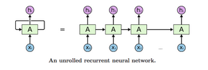
Long Short Term Memory Model, popularly known as LSTM, is a variant of Recurrent Neural Networks (RNNs) that is capable of capturing the long term dependencies in the input sequence. LSTM has a wide range of applications in Sequence-to-Sequence modeling tasks like Speech Recognition, Text Summarization, Video Classification, and so on.

A Long Short Term Memory Node

Let’s discuss in detail how we can train our model using these two approaches.

Wavenet: The Training Phase

This is a Many-to-One problem where the input is a sequence of amplitude values and the output is the subsequent value.

Let’s see how we can prepare input and output sequences.

Input to the WaveNet

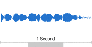
WaveNet takes the chunk of a raw audio wave as an input. Raw audio wave refers to the representation of a wave in the time series domain.

In the time-series domain, an audio wave is represented in the form of amplitude values which are recorded at different intervals of time:

An animated Sound Wave

Output of the WaveNet

Given the sequence of the amplitude values, WaveNet tries to predict the successive amplitude value.

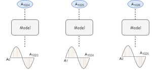
Let’s understand this with the help of an example. Consider an audio wave of 5 seconds with a sampling rate of 16,000 (that is 16,000 samples per second). Now, we have 80,000 samples recorded at different intervals for 5 seconds. Let’s break the audio into chunks of equal size, say 1024 (which is a hyperparameter).

The below diagram illustrates the input and output sequences for the model:

Input and Output of first 3 chunks

We can follow a similar procedure for the rest of the chunks.

We can infer from the above that the output of every chunk depends only on the past information ( i.e. previous timesteps) but not on the future timesteps. Hence, this task is known as Autoregressive task and the model is known as an Autoregressive model.

Inference phase

In the inference phase, we will try to generate new samples. Let’s see how to do that:

Select a random array of sample values as a starting point to model Now, the model outputs the probability distribution over all the samples Choose the value with the maximum probability and append it to an array of samples Delete the first element and pass as an input for the next iteration Repeat steps 2 and 4 for a certain number of iterations

Understanding the WaveNet Architecture

The building blocks of WaveNet are Causal Dilated 1D Convolution layers. Let us first understand the importance of the related concepts.

Why and What is a Convolution?

One of the main reasons for using convolution is to extract the features from an input.

For example, in the case of image processing, convolving the image with a filter gives us a feature map.

In the case of image processing, convolving the image with a filter gives us a feature map

Convolution is a mathematical operation that combines 2 functions. In the case of image processing, convolution is a linear combination of certain parts of an image with the kernel.

You can browse through the below article to read more about convolution:

Architecture of Convolutional Neural Networks (CNNs) Demystified

convolution

1D Convolution

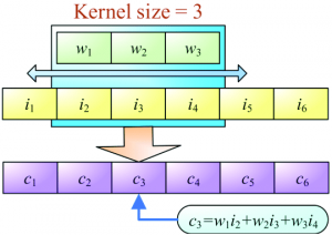
The objective of 1D convolution is similar to the Long Short Term Memory model. It is used to solve similar tasks to those of LSTM. In 1D convolution, a kernel or a filter moves along only one direction:

Calculations involved in a 1D convolution operation

The output of convolution depends upon the size of the kernel, input shape, type of padding, and stride. Now, I will walk you through different types of padding for understanding the importance of using Dilated Causal 1D Convolution layers.

When we set the padding valid, the input and output sequences vary in length. The length of an output is less than an input:

When we set the padding valid, the input and output sequences vary in length. The length of an output is less than an input

When we set the padding to same, zeroes are padded on either side of the input sequence to make the length of input and output equal:

conv

Pros of 1D Convolution

Captures the sequential information present in the input sequence Training is much faster compared to GRU or LSTM because of the absence of recurrent connections Cons of 1D Convolution:

When padding is set to the same, output at timestep t is convolved with the previous t-1 and future timesteps t+1 too. Hence, it violates the Autoregressive principle When padding is set to valid, input and output sequences vary in length which is required for computing residual connections (which will be covered later) This clears the way for the Causal Convolution.

Note: The pros and Cons I mentioned here are specific to this problem.

1D Causal Convolution

This is defined as convolutions where output at time t is convolved only with elements from time t and earlier in the previous layer.

In simpler terms, normal and causal convolutions differ only in padding. In causal convolution, zeroes are added to the left of the input sequence to preserve the principle of autoregressive:

ca

Pros of Causal 1D convolution

Causal convolution does not take into account the future timesteps which is a criterion for building a Generative model Cons of Causal 1D convolution:

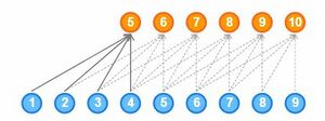
Causal convolution cannot look back into the past or the timesteps that occurred earlier in the sequence. Hence, causal convolution has a very low receptive field. The receptive field of a network refers to the number of inputs influencing an output: causal

As you can see here, the output is influenced by only 5 inputs. Hence, the Receptive field of the network is 5, which is very low. The receptive field of a network can also be increased by adding kernels of large sizes but keep in mind that the computational complexity increases.

Dilated 1D Causal Convolution

A Causal 1D convolution layer with the holes or spaces in between the values of a kernel is known as Dilated 1D convolution.

The number of spaces to be added is given by the dilation rate. It defines the reception field of a network. A kernel of size k and dilation rate d has d-1 holes in between every value in kernel k.

dilated

As you can see here, convolving a 3 * 3 kernel over a 7 * 7 input with dilation rate 2 has a reception field of 5 * 5.

Pros of Dilated 1D Causal Convolution

The dilated 1D convolution network increases the receptive field by exponentially increasing the dilation rate at every hidden layer: conv1d

As you can see here, the output is influenced by all the inputs. Hence, the receptive field of the network is 16.

Residual Block of WaveNet:

A building block contains Residual and Skip connections which are just added to speed up the convergence of the model:

wavenet

The Workflow of WaveNet:

Input is fed into a causal 1D convolution The output is then fed to 2 different dilated 1D convolution layers with sigmoid and tanh activations The element-wise multiplication of 2 different activation values results in a skip connection And the element-wise addition of a skip connection and output of causal 1D results in the residual

Long Short Term Memory (LSTM) Approach Another approach for automatic music generation is based on the Long Short Term Memory (LSTM) model. The preparation of input and output sequences is similar to WaveNet. At each timestep, an amplitude value is fed into the Long Short Term Memory cell – it then computes the hidden vector and passes it on to the next timesteps.

The current hidden vector at timestep ht is computed based on the current input at and previously hidden vector ht-1. This is how the sequential information is captured in any Recurrent Neural Network:

lstm

Pros of LSTM

Captures the sequential information present in the input sequence Cons of LSTM:

It consumes a lot of time for training since it processes the inputs sequentially

Implementation – Automatic Music Generation using Python

The wait is over! Let’s develop an end-to-end model for the automatic generation of music. Fire up your Jupyter notebooks or Colab (or whichever IDE you prefer).

Download the Dataset:

I downloaded and combined multiple classical music files of a digital piano from numerous resources. You can download the final dataset from here.

Import libraries

Music 21 is a Python library developed by MIT for understanding music data. MIDI is a standard format for storing music files. MIDI stands for Musical Instrument Digital Interface. MIDI files contain the instructions rather than the actual audio. Hence, it occupies very little memory. That’s why it is usually preferred while transferring files.

1. library for understanding music

from music21 import * Reading Musical Files:

Let’s define a function straight away for reading the MIDI files. It returns the array of notes and chords present in the musical file.

#defining function to read MIDI files
def read_midi(file):
    
    print("Loading Music File:",file)
    
    notes=[]
    notes_to_parse = None
    
    #parsing a midi file
    midi = converter.parse(file)
  
    #grouping based on different instruments
    s2 = instrument.partitionByInstrument(midi)

    #Looping over all the instruments
    for part in s2.parts:
    
        #select elements of only piano
        if 'Piano' in str(part): 
        
            notes_to_parse = part.recurse() 
      
            #finding whether a particular element is note or a chord
            for element in notes_to_parse:
                
                #note
                if isinstance(element, note.Note):
                    notes.append(str(element.pitch))
                
                #chord
                elif isinstance(element, chord.Chord):
                    notes.append('.'.join(str(n) for n in element.normalOrder))

    return np.array(notes)
view rawmusic_1.py hosted with ❤ by GitHub

Now, we will load the MIDI files into our environment

#for listing down the file names
import os

#Array Processing
import numpy as np

#specify the path
path='schubert/'

#read all the filenames
files=[i for i in os.listdir(path) if i.endswith(".mid")]

#reading each midi file
notes_array = np.array([read_midi(path+i) for i in files])

view rawmusic_2.py hosted with ❤ by GitHub Understanding the data:

Under this section, we will explore the dataset and understand it in detail.

#converting 2D array into 1D array
notes_ = [element for note_ in notes_array for element in note_]

#No. of unique notes
unique_notes = list(set(notes_))
print(len(unique_notes))

view rawmusic_3.py hosted with ❤ by GitHub Output: 304

As you can see here, no. of unique notes is 304. Now, let us see the distribution of the notes.

#importing library
from collections import Counter

#computing frequency of each note
freq = dict(Counter(notes_))

#library for visualiation
import matplotlib.pyplot as plt

#consider only the frequencies
no=[count for _,count in freq.items()]

#set the figure size
plt.figure(figsize=(5,5))

#plot
plt.hist(no)

view rawmusic_4.py hosted with ❤ by GitHub

Output:

music generation

From the above plot, we can infer that most of the notes have a very low frequency. So, let us keep the top frequent notes and ignore the low-frequency ones. Here, I am defining the threshold as 50. Nevertheless, the parameter can be changed.

frequent_notes = [note_ for note_, count in freq.items() if count>=50]
print(len(frequent_notes))
Output: 167

As you can see here, no. of frequently occurring notes is around 170.  Now, let us prepare new musical files which contain only the top frequent notes

new_music=[]

for notes in notes_array:
    temp=[]
    for note_ in notes:
        if note_ in frequent_notes:
            temp.append(note_)            
    new_music.append(temp)
    
new_music = np.array(new_music)

view rawmusic_5.py hosted with ❤ by GitHub

Preparing Data

Preparing the input and output sequences as mentioned in the article:

no_of_timesteps = 32
x = []
y = []

for note_ in new_music:
    for i in range(0, len(note_) - no_of_timesteps, 1):
        
        #preparing input and output sequences
        input_ = note_[i:i + no_of_timesteps]
        output = note_[i + no_of_timesteps]
        
        x.append(input_)
        y.append(output)
        
x=np.array(x)
y=np.array(y)

view rawmusic_6.py hosted with ❤ by GitHub

Now, we will assign a unique integer to every note:

unique_x = list(set(x.ravel()))
x_note_to_int = dict((note_, number) for number, note_ in enumerate(unique_x))
We will prepare the integer sequences for input data

#preparing input sequences
x_seq=[]
for i in x:
    temp=[]
    for j in i:
        #assigning unique integer to every note
        temp.append(x_note_to_int[j])
    x_seq.append(temp)
    
x_seq = np.array(x_seq)

view rawmusic_7.py hosted with ❤ by GitHub Similarly, prepare the integer sequences for output data as well

unique_y = list(set(y))
y_note_to_int = dict((note_, number) for number, note_ in enumerate(unique_y)) 
y_seq=np.array([y_note_to_int[i] for i in y])
Let us preserve 80% of the data for training and the rest 20% for the evaluation:

from sklearn.model_selection import train_test_split
x_tr, x_val, y_tr, y_val = train_test_split(x_seq,y_seq,test_size=0.2,random_state=0)

Model Building

I have defined 2 architectures here – WaveNet and LSTM. Please experiment with both the architectures to understand the importance of WaveNet architecture.

def lstm():
  model = Sequential()
  model.add(LSTM(128,return_sequences=True))
  model.add(LSTM(128))
  model.add(Dense(256))
  model.add(Activation('relu'))
  model.add(Dense(n_vocab))
  model.add(Activation('softmax'))
  model.compile(loss='sparse_categorical_crossentropy', optimizer='adam')
  return model

view rawlstm.py hosted with ❤ by GitHub

I have simplified the architecture of the WaveNet without adding residual and skip connections since the role of these layers is to improve the faster convergence (and WaveNet takes raw audio wave as input). But in our case, the input would be a set of nodes and chords since we are generating music:

from keras.layers import *
from keras.models import *
from keras.callbacks import *
import keras.backend as K

K.clear_session()
model = Sequential()
    
#embedding layer
model.add(Embedding(len(unique_x), 100, input_length=32,trainable=True)) 

model.add(Conv1D(64,3, padding='causal',activation='relu'))
model.add(Dropout(0.2))
model.add(MaxPool1D(2))
    
model.add(Conv1D(128,3,activation='relu',dilation_rate=2,padding='causal'))
model.add(Dropout(0.2))
model.add(MaxPool1D(2))

model.add(Conv1D(256,3,activation='relu',dilation_rate=4,padding='causal'))
model.add(Dropout(0.2))
model.add(MaxPool1D(2))
          
#model.add(Conv1D(256,5,activation='relu'))    
model.add(GlobalMaxPool1D())
    
model.add(Dense(256, activation='relu'))
model.add(Dense(len(unique_y), activation='softmax'))
    
model.compile(loss='sparse_categorical_crossentropy', optimizer='adam')

model.summary()

view raw10_8.py hosted with ❤ by GitHub Define the callback to save the best model during training:

mc=ModelCheckpoint('best_model.h5', monitor='val_loss', mode='min', save_best_only=True,verbose=1)
Let’s train the model with a batch size of 128 for 50 epochs:

history = model.fit(np.array(x_tr),np.array(y_tr),batch_size=128,epochs=50, validation_data=(np.array(x_val),np.array(y_val)),verbose=1, callbacks=[mc])
Loading the best model:

#loading best model
from keras.models import load_model
model = load_model('best_model.h5')
Its time to compose our own music now. We will follow the steps mentioned under the inference phase for the predictions.

import random
ind = np.random.randint(0,len(x_val)-1)

random_music = x_val[ind]

predictions=[]
for i in range(10):

    random_music = random_music.reshape(1,no_of_timesteps)

    prob  = model.predict(random_music)[0]
    y_pred= np.argmax(prob,axis=0)
    predictions.append(y_pred)

    random_music = np.insert(random_music[0],len(random_music[0]),y_pred)
    random_music = random_music[1:]
    
print(predictions)

view raw10_9.py hosted with ❤ by GitHub Now, we will convert the integers back into the notes.

x_int_to_note = dict((number, note_) for number, note_ in enumerate(unique_x)) 
predicted_notes = [x_int_to_note[i] for i in predictions]
The final step is to convert back the predictions into a MIDI file. Let’s define the function to accomplish the task.

def convert_to_midi(prediction_output):
   
    offset = 0
    output_notes = []

    # create note and chord objects based on the values generated by the model
    for pattern in prediction_output:
        
        # pattern is a chord
        if ('.' in pattern) or pattern.isdigit():
            notes_in_chord = pattern.split('.')
            notes = []
            for current_note in notes_in_chord:
                
                cn=int(current_note)
                new_note = note.Note(cn)
                new_note.storedInstrument = instrument.Piano()
                notes.append(new_note)
                
            new_chord = chord.Chord(notes)
            new_chord.offset = offset
            output_notes.append(new_chord)
            
        # pattern is a note
        else:
            
            new_note = note.Note(pattern)
            new_note.offset = offset
            new_note.storedInstrument = instrument.Piano()
            output_notes.append(new_note)

        # increase offset each iteration so that notes do not stack
        offset += 1
    midi_stream = stream.Stream(output_notes)
    midi_stream.write('midi', fp='music.mid')

view raw10_10.py hosted with ❤ by GitHub Converting the predictions into a musical file:

convert_to_midi(predicted_notes) Some of the tunes composed by the model:

Audio Player